The Faddeev-LeVerrier algorithm is one of my favourite algorithms related to linear algebra for a variety of reasons:

It's incredibly elegant
It computes many things at once - the trace of a matrix, its determinant, inverse and the characteristic polynomial (and thus, its eigenvalues).
The task of computing the characteristic polynomial usually requires the use of symbolic computation - one needs to compute $\det(A - \lambda I)$ to get a function of $\lambda$ , while the Faddeev-LeVerrier algorithm can do it numerically.

Initial considerations ⎇

The objective of the Faddeev-LeVerrier algorithm is to compute coefficients of the characteristic polynomial of a square matrix.

$p_{A}(\lambda )\equiv \det(\lambda I_{n}-A)=\sum_{k=0}^{n}c_{k}\lambda ^{k}$

The first observation to be made is that $c_n = 1$ and $c_0 = (-1)^n \det A$ . The algorithm states:

$M_{0} \equiv 0 \\\\ M_{k} \equiv AM_{k-1}+c_{n-k+1}I \\\\ c_{n-k} =-{\frac {1}{k}}\mathrm {tr} (AM_{k}) \\\\$

A few observations assuming a $n$ by $n$ matrix $A$ :

$M_{n+1} = 0$ .
The trace of $A$ is equal to $-c_2$ .
$\det A$ is equal to $(-1)^n c_0$ (a consequence of the previous observations about $c$ ).
$A^{-1}$ is equal to $-\frac{1}{c_0}M_k$ .

An implementation ⎇

I start my implementation by asserting a few things about the environment and the input:

faddeev_leverrier←{
  ⎕io ⎕ml←0 1⋄(≠/⍴⍵)∨2≠≢⍴⍵:⍬
}

I'm interested only in matrices (arrays of rank 2 - 2=≢⍴⍵) and I specifically want them square -=/⍴⍵. If the conditions aren't met, the algorithm returns an empty coefficient vector.

faddeev_leverrier←{
  ⎕io ⎕ml←0 1⋄(≠/⍴⍵)∨2≠≢⍴⍵:⍬
  n←≢⍵⋄M0←⍵⋄I←n n⍴1↑⍨1+n
}

Next up, I define n as the number of rows/columns of the input matrix, M0 as the starting matrix for the algorithm, and I as an identity matrix of order n. The actual recursive implementation of the algorithm will return a vector of the characteristic polynomial coefficients and the matrix corresponding to the current iteration. Since the matrix corresponding to the last iteration is simply n n⍴0 (per observation 1), I will discard it:

faddeev_leverrier←{
  ⎕io ⎕ml←0 1⋄(≠/⍴⍵)∨2≠≢⍴⍵:⍬⋄n←≢⍵
  M0←⍵⋄I←n n⍴1↑⍨1+n⋄⊃ {
    ⍵=0:1 I
  } n
}

I have also added a guard for the final iteration, which simply returns the identity matrix and 1 as the coefficient.

faddeev_leverrier←{
  ⎕io ⎕ml←0 1⋄(≠/⍴⍵)∨2≠≢⍴⍵:⍬⋄n←≢⍵
  M0←⍵⋄I←n n⍴1↑⍨1+n⋄⊃ {
    ⍵=0:1 I⋄(cp MP)←∇⍵-1⋄X←M0+.×MP
  } n
}

I recursively call the function asking for the pair of $M_{n-1}$ and the corresponding c value. I also multiply matrices M0 (the input matrix) and MP (the previous matrix), as it'll prove itself useful in upcoming computations, first one of them being the computation of c for the current iteration. For this purpose, I take the trace of X and divide it by the negated iteration index. The dyadic transposition (axis rearrangement) 0 0⍉X yields the leading diagonal of X, while +/ sums it.

faddeev_leverrier←{
  ⎕io ⎕ml←0 1⋄(≠/⍴⍵)∨2≠≢⍴⍵:⍬⋄n←≢⍵
  M0←⍵⋄I←n n⍴1↑⍨1+n⋄⊃ {
    ⍵=0:1 I⋄(cp MP)←∇⍵-1⋄X←M0+.×MP
    c←(+/0 0⍉X)÷-⍵
  } n
}

I am one step away from the final version of the algorithm, the only thing left is returning the result tuple:

faddeev_leverrier←{
  ⎕io ⎕ml←0 1⋄(≠/⍴⍵)∨2≠≢⍴⍵:⍬⋄n←≢⍵
  M0←⍵⋄I←n n⍴1↑⍨1+n⋄⊃ {
    ⍵=0:1 I⋄(cp MP)←∇⍵-1⋄X←M0+.×MP
    c←(+/0 0⍉X)÷-⍵⋄(cp,c)(X+I×c)
  } n
}

The computation of the current M matrix is derived verbatim from the second equation of the algorithm.

Applications ⎇

I will combine today's post with the yesterday's one about polynomial roots. Namely, the yesterday's post already contains an example use of my faddeev_leverrier function. Let's do something different today.

With a few not so beautiful hacks on top of my existing function, I can compute all the properties of my test matrix:

faddeev_leverrier←{
  ⎕io ⎕ml←0 1⋄(≠/⍴⍵)∨2≠≢⍴⍵:⍬⋄n←≢⍵
  inv←trace←⍬
  M0←⍵⋄I←n n⍴1↑⍨1+n⋄cpoly←⊃ {
    ⍵=0:1 I⋄(cp MP)←∇⍵-1⋄X←M0+.×MP
    c←(+/0 0⍉X)÷-⍵
    MC←X+I×c
    _←{⍵=n-1:inv∘←MC⋄0}⍵
    _←{⍵=1:trace∘←-c⋄0}⍵
    (cp,c)MC
  } n
  (inv×-÷⊃⌽cpoly) trace cpoly ((⊃⌽cpoly)×¯1*n)
}

The function will return a vector of:

inverse matrix
trace
characteristic polynomial
determinant

  data
3 1 5
3 3 1
4 6 4
  faddeev_leverrier data
┌─────────────────┬──┬───────────┬──┐
│ 0.15  0.65 ¯0.35│10│1 ¯10 4 ¯40│40│
│¯0.2  ¯0.2   0.3 │  │           │  │
│ 0.15 ¯0.35  0.15│  │           │  │
└─────────────────┴──┴───────────┴──┘

The results appear to match my pencil and paper calculations (not presented in this blog post - as an exercise, feel free to compute these properties of my test matrix yourself). Of course, there is a way to compute the remaining properties besides the characteristic polynomial using more idiomatic APL:

'alt'⎕cy'dfns'

demo←{
  ⎕io ⎕ml←0 1⋄(≠/⍴⍵)∨2≠≢⍴⍵:⍬
  (⌹⍵) (+/0 0⍉⍵) (-alt× ⍵)
}

The results appear to be the same:

  demo data
┌─────────────────┬──┬──┐
│ 0.15  0.65 ¯0.35│10│40│
│¯0.2  ¯0.2   0.3 │  │  │
│ 0.15 ¯0.35  0.15│  │  │
└─────────────────┴──┴──┘

To my surprise, though, it appears that the Faddeev-LeVerrier algorithm is faster for this particular test case! The benchmark data:

      cmpx 'demo data' 'faddeev_leverrier data'
  demo data              → 2.7E¯5 |   0% ⎕⎕⎕⎕⎕⎕⎕⎕⎕⎕⎕⎕⎕⎕⎕⎕⎕⎕⎕⎕⎕⎕⎕⎕⎕⎕⎕⎕⎕⎕⎕⎕⎕⎕⎕⎕⎕⎕⎕⎕
* faddeev_leverrier data → 1.5E¯5 | -45% ⎕⎕⎕⎕⎕⎕⎕⎕⎕⎕⎕⎕⎕⎕⎕⎕⎕⎕⎕⎕⎕⎕                
      demo data
┌─────────────────┬──┬──┐
│ 0.15  0.65 ¯0.35│10│40│
│¯0.2  ¯0.2   0.3 │  │  │
│ 0.15 ¯0.35  0.15│  │  │
└─────────────────┴──┴──┘
      faddeev_leverrier data
┌─────────────────┬──┬───────────┬──┐
│ 0.15  0.65 ¯0.35│10│1 ¯10 4 ¯40│40│
│¯0.2  ¯0.2   0.3 │  │           │  │
│ 0.15 ¯0.35  0.15│  │           │  │
└─────────────────┴──┴───────────┴──┘

Replacing the generalised alternant with a (hopefully) more performant determinant function yields oddly similar results:

      cmpx 'demo data' 'faddeev_leverrier data'
  demo data              → 2.0E¯5 |   0% ⎕⎕⎕⎕⎕⎕⎕⎕⎕⎕⎕⎕⎕⎕⎕⎕⎕⎕⎕⎕⎕⎕⎕⎕⎕⎕⎕⎕⎕⎕⎕⎕⎕⎕⎕⎕⎕⎕⎕⎕
* faddeev_leverrier data → 1.5E¯5 | -25% ⎕⎕⎕⎕⎕⎕⎕⎕⎕⎕⎕⎕⎕⎕⎕⎕⎕⎕⎕⎕⎕⎕⎕⎕⎕⎕⎕⎕⎕⎕

Eigenvectors ⎇

The final part of my blog post will shed some more light on eigenvectors. Let's compute the eigenvalues first:

  50 solve faddeev_leverrier data
0J2 0J¯2 10

For simplicity, I will present the pencil and paper calculations for $\lambda = 10$ alongside the APL code. I start with computing $A - \lambda I$ :

eigenvec←{
  ⎕io ⎕ml←0 1⋄(≠/⍴⍵)∨2≠≢⍴⍵:⍬
  n←≢⍵⋄I←n n⍴1↑⍨1+n⋄s←⍵-⍺×I
}

$A - \lambda I = \begin{vmatrix} -7 & 1 & 5\\\\ 3 & -7 & 1\\\\ 4 & 6 & -6 \end{vmatrix}$

$(A - \lambda I) \cdot v = 0$ yields a homogenous equation system which needs to be solved. A very sad property of this system is that it's underspecified, so $x_{k-1}$ up to $n$ are all functions of $x_n$ . Surprisingly, that's not a problem, though! If we ignore the presence of $x_n$ , turns out one row of the matrix is redundant. If we assume that $x_n = 1$ , in our example, we solve a non-homogenous system of equations with two variables.

eigenvec←{
  ⎕io ⎕ml←0 1⋄(≠/⍴⍵)∨2≠≢⍴⍵:⍬
  n←≢⍵⋄I←n n⍴1↑⍨1+n⋄s←⍵-⍺×I
  N←{¯9 ¯11+.○(⊢×⎕ct<|)9 11∘.○⍵}
  q←1,⍨1↑⍨1-⍨⊃⌽⍴s⋄N¨1,⍨∊⌹⍨∘-/q⊂1↓s
}

$x_1 = \frac{18}{23} \\\\ x_2 = \frac{11}{23} \\\\ x_3 = 1$

Of course, one could scale $x_3$ as they please, and modify $x_1$ and $x_2$ accordingly. I also use the same real/imaginary truncation technique as outlined in the previous post to strip (likely) unnecessary real/imaginary parts. Finally, I test my code:

  data∘(eigenvec⍨)¨ 50 solve faddeev_leverrier data
┌───────────┬───────────┬───────────────────────────┐
│¯1J¯1 0J1 1│¯1J1 0J¯1 1│0.7826086957 0.4782608696 1│
└───────────┴───────────┴───────────────────────────┘

The results seem to match. Great!

Summary ⎇

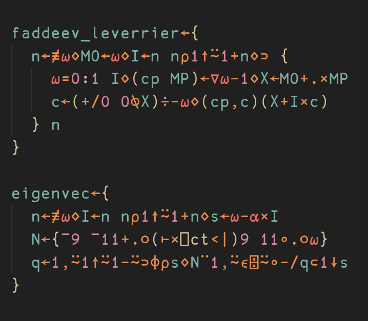
I believe that today's post was much more involved than the previous ones. The full source code follows:

faddeev_leverrier←{
  ⎕io ⎕ml←0 1⋄(≠/⍴⍵)∨2≠≢⍴⍵:⍬⋄n←≢⍵
  M0←⍵⋄I←n n⍴1↑⍨1+n⋄⊃ {
    ⍵=0:1 I⋄(cp MP)←∇⍵-1⋄X←M0+.×MP
    c←(+/0 0⍉X)÷-⍵⋄(cp,c)(X+I×c)
  } n
}

demo←{
  ⎕io ⎕ml←0 1⋄(≠/⍴⍵)∨2≠≢⍴⍵:⍬
  (⌹⍵) (+/0 0⍉⍵) (-alt× ⍵)
}

⍝ A less general version that uses det instead.
demo←{
  ⎕io ⎕ml←0 1⋄(≠/⍴⍵)∨2≠≢⍴⍵:⍬
  (⌹⍵) (+/0 0⍉⍵) (det ⍵)
}

eigenvec←{
  ⎕io ⎕ml←0 1⋄(≠/⍴⍵)∨2≠≢⍴⍵:⍬
  n←≢⍵⋄I←n n⍴1↑⍨1+n⋄s←⍵-⍺×I
  N←{¯9 ¯11+.○(⊢×⎕ct<|)9 11∘.○⍵}
  q←1,⍨1↑⍨1-⍨⊃⌽⍴s⋄N¨1,⍨∊⌹⍨∘-/q⊂1↓s
}

⍝ Alternatively, the "more powerful" Faddeev-LeVerrier algorithm implementation.
faddeev_leverrier←{
  ⎕io ⎕ml←0 1⋄(≠/⍴⍵)∨2≠≢⍴⍵:⍬⋄n←≢⍵
  inv←trace←⍬
  M0←⍵⋄I←n n⍴1↑⍨1+n⋄cpoly←⊃ {
    ⍵=0:1 I⋄(cp MP)←∇⍵-1⋄X←M0+.×MP
    c←(+/0 0⍉X)÷-⍵
    MC←X+I×c
    _←{⍵=n-1:inv∘←MC⋄0}⍵
    _←{⍵=1:trace∘←-c⋄0}⍵
    (cp,c)MC
  } n
  (inv×-÷⊃⌽cpoly) trace cpoly ((⊃⌽cpoly)×¯1*n)
}

Implementing the Faddeev-LeVerrier algorithm in APL

Initial considerations ⎇

An implementation ⎇

Applications ⎇

Eigenvectors ⎇

Summary ⎇