iczelia :: Heaviside's partial fraction decomposition method.

Introduction ⎇

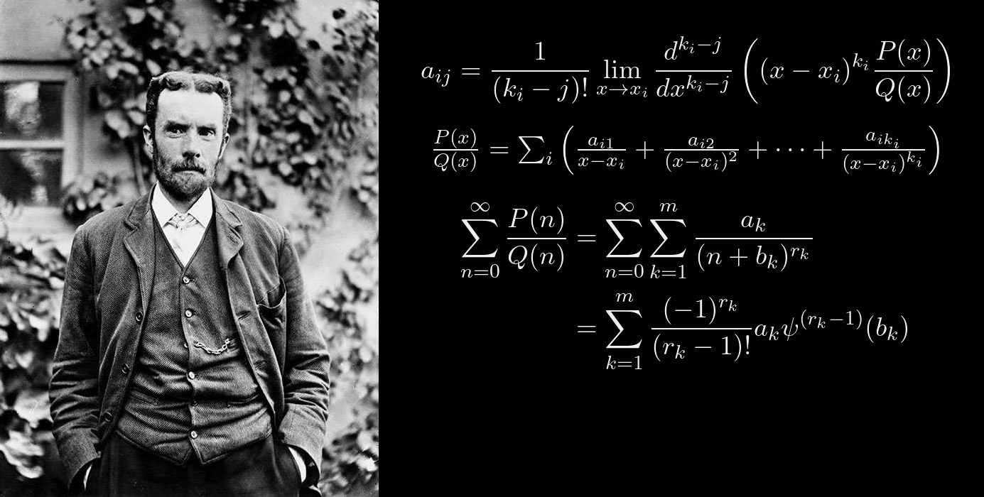
In high school algebra, it is demonstrated that a rational function (a quotient of two polynomial functions) can be expressed as the sum of partial fractions, which are terms of the form

$\frac{A}{(x-x_0)^k}$

The importance of the partial fraction decomposition lies in the fact that it provides algorithms for various computations with rational functions, including the explicit computation of antiderivatives (discussed later in the blog post), Taylor series expansions and inverse Laplace transforms.

In this blog post, I assume that $\deg P \le \deg Q$ , i.e. that the denominator has a lower degree than the numerator. Otherwise, one can use Euclidean division and seek partial fractions of $R(x) / Q(x)$ , where $R(x)$ is the remainder of the division guaranteed to have a lower degree of $Q$ .

The high school method ⎇

Consider the following function:

$\frac{s^2-2s+1}{s(s-2)^2(s^2+1)} = \frac{A}{s} + \frac{B}{s-2} + \frac{C}{(s-2)^2} + \frac{Ds + E}{s^2+1}$

We clear the fractions, i.e. multiply both sides by the denominator:

$s^2-2s+1=A(s-2)^2(s^2+1) + Bs(s-2)(s^2+1) + Cs(s^2+1) + (Ds + E)s(s-2)^2$

Clearly, $A = 0.25$ (found by substituting $0$ ). Substituting $2$ tells us that $C=0.1$ . Consequently, $B=0.07$ . Finally, $D = 0.32$ and $E = 0.24$ . Hence:

$\frac{s^2-2s+1}{s(s-2)^2(s^2+1)} = \frac{0.25}{s} + \frac{0.07}{s-2} + \frac{0.1}{(s-2)^2} + \frac{0.32s + 0.24}{s^2+1}$

Clearly, this method is very tedious and difficult to automate (the algorithm needs the ability to simplify and extensively manipulate rational functions).

Heaviside method ⎇

The Heaviside method in the base case can deal only with rational functions, the denominators of which do not contain any repeated roots. To illustrate the intuition behind this method, consider the following function:

$\frac{2s+1}{s(s-1)(s+1)} = \frac{A}{s} + \frac{B}{s-1} + \frac{C}{s+1}$

Olivier Heaviside proposes to find the value of $C$ by covering the $s+1$ term and substituting $s=-1$ :

$\frac{2s+1}{s(s-1)\color{transparent}{(s+1)}} \Bigg|_{-1} = \frac{C}{\color{transparent}{s+1}}$

Clearly, $C = 0.5$ . To justify this maneuver, multiply both sides by $s+1$ in the original expression:

$\frac{(2s+1)(s+1)}{s(s-1)(s+1)} = \frac{A(s+1)}{s} + \frac{B(s+1)}{s-1} + \frac{C(s+1)}{s+1}$

After a chain of simplifications the problem reduces to the following:

$\frac{(2s+1)}{s(s-1)} = \frac{A(s+1)}{s} + \frac{B(s+1)}{s-1} + C$

Setting $s = -1$ annihilates the first two terms on the right-hand side, and the result follows:

$\frac{(2s+1)}{s(s-1)} \Bigg|_{-1} = C$

Most textbooks, courses and online resources stop here, but the method can also be extended to rational functions with repeated roots.

Domain extension ⎇

The basic idea is factoring out the repeated roots and recursing (with memoisation) as follows:

$\begin{aligned} f(s) &= \frac{1}{(s-1)^2(s-2)}\\\\ &= \frac{1}{s-1} \left(\frac{1}{(s-1)(s-2)}\right)\\\\ &= \frac{1}{s-1} \left(\frac{1}{s-2} - \frac{1}{s-1}\right) && \text{by Heaviside}\\\\ &= \frac{-1}{(s-1)^2} + \frac{1}{(s-1)(s-2)}\\\\ &= \frac{-1}{(s-1)^2} + \frac{1}{s-2} - \frac{1}{s-1} && \text{by Heaviside} \end{aligned}$

Before we allow repeated roots, we must assume that the polynomial $Q(x) \in F[x]$ does not have factors that are irreducible over $F$ . This is not an unreasonable demand, as the polynomial can often be solved numerically.

Over the complex field, the rational function is by definition factored as follows:

$f(x)=\sum_{i}\left({\frac {a_{i1}}{x-x_{i}}}+{\frac {a_{i2}}{(x-x_{i})^{2}}}+\cdots +{\frac {a_{ik_{i}}}{(x-x_{i})^{k_{i}}}}\right)$

Let $g_{ij}(x)=(x-x_{i})^{j-1}f(x)$ . Then, according to the uniqueness of Laurent series, $a_{ij}$ is the coefficient of the term $(x − x_i)^{−1}$ in the Laurent expansion of $g_{ij}(x)$ about the point $x_i$ , i.e., its residue $a_{ij}=\operatorname {Res} (g_{ij},x_{i})$ .

This is given by the formula:

$a_{ij}={\frac {1}{(k_{i}-j)!}}\lim_{x\to x_{i}}{\frac {d^{k_{i}-j}}{dx^{k_{i}-j}}}\left((x-x_{i})^{k_{i}}\frac{P(x)}{Q(x)}\right)$

When $x_i$ is a root with multiplicity of one, the formula reduces to:

$a_{i1}={\frac {P(x_{i})}{Q'(x_{i})}}$

Consistently with Lagrange interpolation.

Improvements to the formula ⎇

Unfortunately, Heaviside's original approach requires successive differentiation. This can be avoided in the following way:

Consider the following derivation for the partial fraction's last term of a given root (given $k_i$ as the multiplicity of the $i$ -th unique root $x_i$ ):

$a_{i k_{i}}=\lim_{x \to x_i} f(x) (x-x_i)^{k_i}$

By multiplying both sides of the definition by $(x - x_i)^{k_i}$ , we cancel out the $(x - x_i)$ factor in $Q(x)$ and include $(x - x_i)$ or its higher power in each partial fraction, except the constant term $a_{i k_i}$ .

Consider the following function:

$\frac{P_{i1}(x)}{Q_{i1}(x)} = \frac{P(x)}{Q(x)} - \frac{a_{i k_i}}{(x - x_i)^{k_i}}$

Due to the uniqueness of the partial fraction expansion, the highest power of $(x - x_i)$ in $Q_{i1}(x)$ is $k_i-1$ , further implying that $(x - x_i)$ must be cancelled out when simplifying $\frac{P_{i1}(x)}{Q_{i1}(x)}$ . Thus, we can reduce the multiplicity of the pole at $x_i$ by one via a single polynomial division. By applying the technique again, we can determine $a_{i k_{i-1}}$ readily:

$a_{i k_{i-1}} = \lim_{x \to x_i} \frac{P_{i1}(x)}{Q_{i1}(x)} (x-x_i)^{k_i-1}$

As such, we consider:

$\frac{P_{ij}(x)}{Q_{ij}(x)} = \frac{P(x)}{Q(x)} - \sum_{m=0}^{j-1} \frac{a_{i k_i-m}}{(x - x_i)^{k_i-m}}$

To determine the formula for $a_{i k_i-j}$ for $i \in [1, s]$ ( $s$ being the amount of unique roots) and $j \in [1, k_i-1]$ , proceed as:

$a_{i k_i-j} = \lim_{x \to x_i} \frac{P_{ij}(x)}{Q_{ij}(x)} (x-x_i)^{k_i-j} = \lim_{x \to x_i} \left(\frac{P(x)}{Q(x)} - \sum_{m=0}^{j-1} \frac{a_{i k_i-m}}{(x - x_i)^{k_i-m}}\right) (x-x_i)^{k_i-j}$

An example ⎇

We want to find the partial fractions of the following function:

$\frac{2x+1}{x(x-1)(x-2)^2} = \frac{A}{x} + \frac{B}{x-1} + \frac{C}{x-2} + \frac{D}{(x-2)^2}$

Applying the first step to $A$ , $B$ and $D$ yields:

$$ \begin{aligned} A &= \lim_{x\to x_i} f(x) (x-x_i)^{k_i} && \text{by definition} \\\\ &= \lim_{x\to 0} f(x) x && \text{by values of $x_1$ and $k_1$ } \\\\ &= \lim_{x\to 0} \frac{x(2x+1)}{x(x-1)(x-2)^2} && \text{by definition of $f$ } \\\\ &= \lim_{x\to 0} \frac{(2x+1)}{(x-1)(x-2)^2} && \text{cancel out $x$ } \\\\ &= \frac{1}{(0-1)(0-2)^2} && \text{substitute into the limit} \\\\ &= -\frac{1}{4} \\\\ B &= \lim_{x\to x_i} f(x) (x-x_i)^{k_i} = \lim_{x\to 1} f(x) (x-1) \\\\ &= \lim_{x\to 1} \frac{(x-1)(2x+1)}{x(x-1)(x-2)^2} = \lim_{x\to 1} \frac{(2x+1)}{x(x-2)^2} \\\\ &= \frac{2+1}{(1-2)^2} = 3 \\\\ D &= \lim_{x\to x_i} f(x) (x-x_i)^{k_i} = \lim_{x\to 2} f(x) (x-2)^2 \\\\ &= \lim_{x\to 2} \frac{(x-2)^2(2x+1)}{x(x-1)(x-2)^2} = \lim_{x\to 2} \frac{(2x+1)}{x(x-1)} \\\\ &= \frac{(4+1)}{2} = 2.5 \end{aligned} $$

The value of $C = a_{31}$ is calculated by considering the formula for $a_{i k_i-j}$ with $i = 3$ , $k_i = 2$ , $j = 1$ and $x_i = 2$ :

$\begin{aligned} C = a_{31} &= \lim_{x \to 2} \frac{P_{31}(x)}{Q_{31}(x)} (x-2) \\\\ &= \lim_{x \to 2} \left(\frac{P(x)}{Q(x)} - \frac{a_{32}}{(x - 2)^{2}}\right) (x-2) \\\\ &= \lim_{x \to 2} \left(\frac{2x+1}{x(x-1)(x-2)^2} - \frac{2.5}{(x - 2)^{2}}\right) (x-2) \\\\ &= \lim_{x \to 2} \frac{2x+1}{x(x-1)(x-2)} - \frac{2.5}{(x - 2)} \\\\ &= \lim_{x \to 2} \frac{-2.5x-0.5}{x(x-1)} \\\\ &= -2.75 \end{aligned}$

Hence, the partial fraction decomposition follows as:

$\frac{2x+1}{x(x-1)(x-2)^2} = \frac{-0.25}{x} + \frac{3}{x-1} + \frac{-2.75}{x-2} + \frac{2.5}{(x-2)^2}$

Application to antiderivatives ⎇

Partial fraction decomposition, especially when performed using this simple algorithm can be used to compute antiderivatives and infinite sums of rational functions.

Consider this motivating example:

$\int \dfrac{3x^4+ 4x^3 + 3x^2}{(x+6)(x-7)(x-3)^2} \mathrm dx = \int \frac{4361}{104 (x-7)} - \frac{21}{2(x-3)^2} - \frac{335}{24 (x-3)} - \frac{116}{39 (x+6)} + 3 \mathrm dx$

Which is trivially computed using a elementary integration techniques, starting with a rule to break up the expression into parts:

$\displaystyle \int f(x)+g(x) \mathrm dx = \int f(x) \mathrm dx + \int g(x) \mathrm dx$

Then, each expression following the same rule is integrated as follows:

$\displaystyle \int \frac{a}{(x-b)^n} \mathrm dx = \frac{a(x-b)^{1-n}}{1-n} + C$

An alternative way to approach problems like these is using the Ostrogradsky-Hermite's method. Consider the following integral:

$I=\int \dfrac{27x^8+18x^7-23x^6+15x^5-99x^4+3x^3+2x^2+10x-5}{5x^7-63x^6+267x^5-349x^4-324x^3+912x^2-448x} \mathrm dx$

We begin by finding $Q'(x)$ as follows:

$Q'(x) = (x-4)^2 (35x^4-98x^3-9x^2+100x-28)$

Then, it becomes apparent that

$\text{gcd}(Q, Q') = Q_1 = (x-4)^2(x-1)$

We find $Q_2$ as follows:

$Q_2 = \frac{Q}{Q_1} = 5 x^4 - 18 x^3 - 15 x^2 + 28 x$

$P_1(x)$ and $P_2(x)$ are currently unknown, but they will have degrees one less than those of $Q_1(x)$ and $Q_2(x)$ , respectively. Thus:

$I=\frac{ax^3+bx^2+cx+d}{5 x^4 - 18 x^3 - 15 x^2 + 28 x}+\int \frac{ex^3+fx^2+gx+h}{5 x^4 - 18 x^3 - 15 x^2 + 28 x} \mathrm dx$

The merit of this method is obvious: The integral of a rational function which has roots with non-one multiplicity was reduced to an integral of a rational function with simple roots, akin to the domain extension to the Heaviside method. The coefficients must be equated now to find the values from $a$ to $h$ , which is a rather tedious and simple task left to a determined reader.

Application to infinite sums ⎇

The following identity involving the polygamma function can be used to compute infinite sums of rational functions:

$\sum_{n=0}^{\infty}\frac{P(n)}{Q(n)}=\sum_{n=0}^{\infty}\sum_{k=1}^{m}{\frac{a_{k}}{(n+b_{k})^{r_{k}}}}=\sum_{k=1}^{m}{\frac{(-1)^{r_{k}}}{(r_{k}-1)!}}a_{k}\psi ^{(r_{k}-1)}(b_{k})$

The second term is a partial fraction decomposition of the rational function, which can be computed using methods described earlier. The notation $\psi ^{(a)}(x)$ denotes the polygamma function of the $a$ -th order, defined as the $a$ -th derivative of the digamma function, the logarithmic derivative of $\Gamma(x)$ . While in this scenario $a>0$ and $a\in \mathbb{N}$ is almost taken for granted, the following formula can be used to compute the polygamma function also given that $\Re z > 0$ :

${\begin{aligned}\psi ^{(m)}(z)&=(-1)^{m+1}\int _{0}^{\infty }{\frac {t^{m}e^{-zt}}{1-e^{-t}}}\mathrm {d} t\\\\&=-\int _{0}^{1}{\frac {t^{z-1}}{1-t}}(\ln t)^{m}\mathrm {d} t\\\\&=(-1)^{m+1}m!\zeta (m+1,z)\end{aligned}}$

If $a = 0$ and $\Re z > 0$ , then:

$\psi(z) = \int_0^\infty {\frac {e^{-t} } t - \frac {e^{-z t} } {1 - e^{-t} } } \mathrm dt$

If $z$ is outside of the domain, this is easily fixed using the digamma reflection formula: $\psi (1-x)-\psi (x)=\pi \cot \pi x$

Meanwhile the same defect with the general formula is fixed using the polygamma reflection formula: $(-1)^{m}\psi ^{(m)}(1-z)-\psi ^{(m)}(z)=\pi {\frac {\mathrm {d} ^{m}}{\mathrm {d} z^{m}}}\cot {\pi z}=\pi ^{m+1}{\frac {P_{m}(\cos {\pi z})}{\sin ^{m+1}(\pi z)}}$

Given that:

${\begin{aligned}P_{0}(x)&=x\\\\P_{m+1}(x)&=-\left((m+1)xP_{m}(x)+\left(1-x^{2}\right)P'_{m}(x)\right)\end{aligned}}$

Conclusion ⎇

The Heaviside method is a simple and elegant way to compute partial fraction decompositions of rational functions. Researching this topic has been a very interesting experience, and I hope that this blog post will be useful to someone who is also dealing with real and complex analysis in computer algebra.